Cryptoucan™ PCB visual control
Basic computer vision algorithms may aid you in performing visual control of whatever you may be manufacturing. But if you want something more, you need to turn to the magic world of … linear algebra. Read on to see how all those little vectors and matrices help us with QA.
Even though our testing devices are equipped with camera of extraordinary resolution, it is not wise to rely on extremely precise positioning of the PCB[1] holder and the camera arm. Therefore we have a special aiming markers – consisting of concentric circles – on our PCB and using computer vision[2] algorithms we find their centers. Of course, the circle finding algorithm – as mentioned last week[3] – may find more circles depending on the lighting conditions. Yet as the algorithm knows where about to find the markers, it can easily discard false positives and we have their positions in camera coordinates.
We also have the coordinates of these reference points in the model of our PCB and with known locations in both coordinate systems, it is pretty easy to convert between these two. Let’s dissect the algorithm in its purest form. We denote the first marker $A$ and the second $B$. For camera coordinate system we use the notation $A’$ and $B’$. We will also denote all 2D coordinates as normalized vectors of size 3, like:
$A=\pmatrix{A_x\\A_y\\1}$
As the first step, we move the source coordinate system so that the origin $O=[0,0]$ lies at the position of the first marker. Like this:
$X_1=X-A$
The second step should adjust the scale. To achieve this, we calculate the vector from point $A’$ to point $B’$ and the same vector from point $A$ to point $B$. Their ratio is the scale ratio we are looking for:
$\Delta=B-A$
$\Delta’=B‘-A’$
$s=\frac{|\Delta’|}{|\Delta|}$
Now, how do we combine the translation and scaling? We need to rewrite the first transformation in normalized $3\times 3$ matrix form:
$M_1=\pmatrix{1&0&-A_x\\0&1&-A_y\\0&0&1}$
The scaling matrix can be written as:
$M_s=\pmatrix{s&0&0\\0&s&0\\0&0&1}$
Combining these two is a simple matter of matrix multiplication:
$M_2=M_s\cdot M_1=\pmatrix{s&0&0\\0&s&0\\0&0&1}\cdot\pmatrix{1&0&-A_x\\0&1&-A_y\\0&0&1}=\begin{pmatrix}s & 0 & -sA_x \\0 & s & -sA_y \\0 & 0 & 1 \\\end{pmatrix}$
Now what with the rotation. Everyone remembers the old rotation[4] by $\alpha$ matrix:
$M_\alpha=\begin{pmatrix}\cos\alpha & -\sin\alpha & 0 \\\sin\alpha & \cos\alpha & 0 \\0 & 0 & 1 \\\end{pmatrix}$
And we know that we need to rotate the coordinate system so $\Delta’$ holds given angle $\beta$ with the X-axis. We actually need to align the vectors $\Delta$ and $\Delta’$ directions and these angles just help us thinking about that. So $\alpha$ is the angle between $\Delta’$ and the X-axis and $\beta$ is the angle between $\Delta$ and – again – the X-axis. If we rotate everything by $-\beta$ and then by $\alpha$, we get the required alignment.
We also know that we can use some trigonometric equivalences here. You can immediately see that:
$\begin{aligned}\cos-\alpha &= \cos\alpha \\
\cos\alpha &= \frac{\Delta_x}{|\Delta|} \\
\sin-\alpha &= -\sin\alpha \\
\sin\alpha &= \frac{\Delta_y}{|\Delta|} \\
-\sin\alpha &= \frac{-\Delta_y}{|\Delta|} \\
\sin-\alpha &= \frac{-\Delta_y}{|\Delta|}\end{aligned}$
The same applies – of course – for $\beta$. So now we can combine the rotation by $-\beta$ and $\alpha$ afterwards:
$M_{-\beta+\alpha}=\begin{pmatrix}
\frac{\Delta’_x}{|\Delta’|} & \frac{-\Delta’_y}{|\Delta’|} & 0 \\
\frac{\Delta’_y}{|\Delta’|} & \frac{\Delta’_x}{|\Delta’|} & 0 \\
0 & 0 & 1 \\
\end{pmatrix}\cdot\begin{pmatrix}
\frac{\Delta_x}{|\Delta|} & \frac{\Delta_y}{|\Delta|} & 0 \\
\frac{-\Delta_y}{|\Delta|} & \frac{\Delta_x}{|\Delta|} & 0 \\
0 & 0 & 1 \\
\end{pmatrix}$
$M_{-\beta+\alpha}=\begin{pmatrix}
\frac{\Delta’_x\Delta_x+\Delta’_y\Delta_y}{|\Delta’|\cdot|\Delta|}
&
\frac{\Delta’_x\Delta_y-\Delta’_y\Delta_x}{|\Delta’|\cdot|\Delta|}
&
0
\\
\frac{\Delta’_y\Delta_x-\Delta’_x\Delta_y}{|\Delta’|\cdot|\Delta|}
&
\frac{\Delta’_y\Delta_y+\Delta’_x\Delta_x}{|\Delta’|\cdot|\Delta|}
&
0
\\
0 & 0 & 1 \\
\end{pmatrix}$
This looks rather ugly, therefore we use another simple substitution:
$ \begin{aligned}
m &= \frac{\Delta’_x\Delta_x+\Delta’_y\Delta_y}{|\Delta’|\cdot|\Delta|} \\
n &= \frac{\Delta’_x\Delta_y-\Delta’_y\Delta_x}{|\Delta’|\cdot|\Delta|}
\end{aligned}$
And now we can rewrite the whole rotation as:
$M_{-\beta+\alpha}=\begin{pmatrix}
m & -n & 0 \\
n & m & 0 \\
0 & 0 & 1 \\
\end{pmatrix}$
Last part is moving the origin $O$ to point $A$:
$M_3=\pmatrix{1&0&A’_x\\0&1&A’_y\\0&0&1}$
Of course, we can join it with already derived transformations:
$M=M_3\cdot M_{-\beta+\alpha}\cdot M_2$
$M=\pmatrix{1&0&A’_x\\0&1&A’_y\\0&0&1}\cdot\begin{pmatrix}
m & -n & 0 \\
n & m & 0 \\
0 & 0 & 1 \\
\end{pmatrix}\cdot\begin{pmatrix}s & 0 & -sA_x \\0 & s & -sA_y \\0 & 0 & 1 \\\end{pmatrix}$
$M=\begin{pmatrix}
ms & -ns & -msA_x+nsA_y \\
ns & ms & -nsA_x-msA_y \\
0 & 0 & 1 \\
\end{pmatrix}$
Yes, there are few tricks involved I did not show you – but you can easily derive them yourself. For example there is no need for calculating the sizes of $\Delta$ and $\Delta’$ – therefore you can save calculating the square roots there. The resulting transformation can be pretty fast and can be performed in real time even on a slower computer. You can see the accuracy in Picture 1 below.
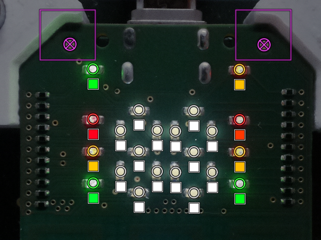
Picture 1: Coordinate system transformation in real QA application (including LED color checking)
The program is – of course – not just a simple coordinates transformation. There is also color-space transformation in place which helps us check the intensity and correct color of every LED soldered.
Thank you for staying with us and I hope we have proven we take the quality control seriously. Come back next week for more!
References
1. Wikipedia contributors. (2018, December 5). Printed circuit board. In Wikipedia, The Free Encyclopedia. Retrieved 20:39, December 5, 2018, from https://en.wikipedia.org/w/index.php?title=Printed_circuit_board&oldid=872176800
2. Wikipedia contributors. (2018, November 27). Computer vision. In Wikipedia, The Free Encyclopedia. Retrieved 20:40, December 5, 2018, from https://en.wikipedia.org/w/index.php?title=Computer_vision&oldid=870818488
3. https://trustica.cz/en/2018/11/29/cryptoucan-pcb-quality-control/
4. Wikipedia contributors. (2018, November 15). Rotation. In Wikipedia, The Free Encyclopedia. Retrieved 20:41, December 5, 2018, from https://en.wikipedia.org/w/index.php?title=Rotation&oldid=868935494