Numerical approximation of inverse functions in Racket

In one of our recent projects we are working hard to be able to detect filesystem changes that may indicate substantiate increase in the number of encrypted files. There may be several hints that given file contains encrypted data and one of the most prominent properties of such file is its high entropy. But how to measure it? And how to measure it effectively? In this post we will look into a relatively simple statistical analysis of file data that can shed light on its entropy. The only problem here is there are no readily available software solutions to do this.

If you look at typical data as a chunk of bytes you can tell high-entropy data by checking the statistical distribution of all possible byte values within that chunk. Sounds a bit cryptic? It is not that hard. As byte is eight bits wide it can store values from 0 to 255 (that is 2^8-1). So for some block of bytes there should be roughly the same number of each possible values. For example for a block of 2560 bytes each possible value should be present about ten times.

How to measure how much given block deviates from this ideal random distribution? You can use what statisticians call a chi-squared test. The good thing about chi-squared distribution is that when you add combine data of this distribution you can also use addition of deviations from distribution of each element and get a value that tells you about deviation of such combined distribution. The number of distributions you combine is usually called the distribution's degrees of freedom - that is how many independent elements you examine. Then you can calculate the sum of chi-squared errors and compare it to expected value at given probability level.

The probability level is an important variable that tells us how many test will give false positive results. It is usually assumed that this probability level - called P-value for short - around 5% is sufficient for real-world testing scenarios. 5% means that one in twenty tests that give positive result may actually be negative. For our testing we chose to compensate for this property by testing multiple blocks and check how many pass the test. If enough blocks pass the chi-squared test, we may safely assume the file composed of these blocks has a high entropy and therefore has a high probability of being encrypted.

There was just one downside. Calculating the chi-squared sum for given data block is easy. But getting the value to compare the result to turned out to be a bit problematic. There are tables that list these values but as these are usually used in non-binary scenarios and we have 256 degrees of freedom we were unable to find a definite source for the threshold value.

So how do we calculate the threshold value for 256 degrees of freedom and 5% P-value?

The answer lies in the mathematics underneath. It is simply a value of inverse cumulative distribution function for 256 degrees of freedom and P-value of 5% which cannot be obtained analytically. The cumulative distribution function can be computed analytically so we started with that. As the project programming language is Racket (http://www.racket-lang.org/), we were able to use available scientific library for calculating values of this function.

(require (planet williams/science/random-distributions))
(displayln (chi-squared-cdf x 256))

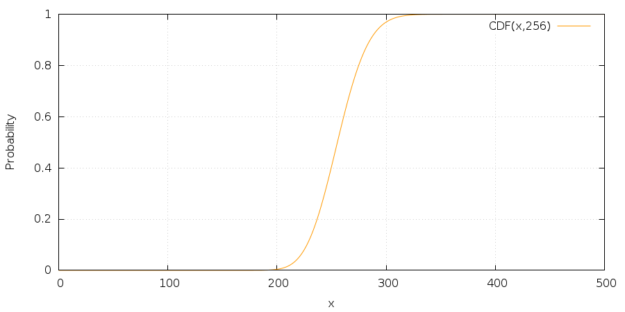
Which displays the value for given 'x'. It seemed easy enough and so we plotted the values into a graph we could comprehend:

But we needed an inverse function and as mentioned above it is not possible to get a simple analytical representation. Therefore we used an range-halving and range-extending algorithm to pin-point approximate value for our application. The algorithm is pretty simple and resembles well-known algorithms used for approximating square roots and similar functions:

(define (chi-squared-inverse-cdf p df)
  (let ((one-p (- 1 p))
        (convergence (/ p 1000000 df)))
    (define (loop x^2-lower x^2-upper)
      (let* ((x^2-mid (+ x^2-lower (/ (- x^2-upper x^2-lower) 2)))
             (cdf (chi-squared-cdf x^2-mid df)))
        (if (and (> cdf one-p)
                 (< (- cdf one-p) convergence))
            x^2-mid
            (cond
              ((&gt; cdf one-p)
               (loop x^2-lower x^2-mid))
              ((< cdf one-p)
               (let ((cdf-upper (chi-squared-cdf x^2-upper df)))
                 (if (< cdf-upper one-p)
                     (loop x^2-mid
                       (+ x^2-upper (* (- x^2-upper x^2-lower) 2)))
                     (loop x^2-mid x^2-upper))))))))
    (loop 0 1)))

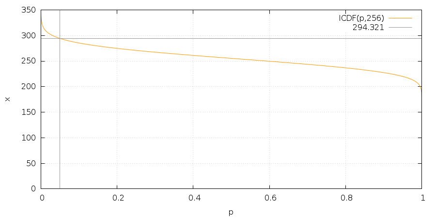
Just to be sure we also plotted the graph of the resulting function and it looked fine:

And that is it. In case you need it without the hard math or programming, the right value for 256 degrees of freedom at the 5% probability level is roughly 294.321.

I hope this was not way too much mathematically boring but you enjoyed it at least a bit.

Cheers!